Many of you rely on spreadsheets (csv or xlsx) to import your data into Kumu. Sometimes your data is ready to go and doesn't require much cleaning or finagling. Other times that isn't the case.
For those times when it starts to feel like you're losing the battle to your spreadsheet, here's your guide to the essential formulas, features and tricks for coming out on top.
Note: These instructions are geared towards users of Microsoft Excel but should align pretty close if you are using Google Sheets instead.
1. Use conditional formatting to detect duplicates and blank cells
If you're working with data that hasn't been cleaned, you can easily run into an import spreadsheet that has the same element listed multiple times. This can cause some havoc when you import.
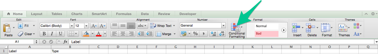
With conditional formatting, you can quickly create a rule to highlight duplicate values (or blanks). First select the column of your spreadsheet that contains the element labels. If you are on the "home" tab of the Excel ribbon, you'll see a conditional formatting button:
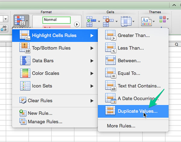
Then simply choose "highlight cells rules" and then "duplicate values", choose the coloring you'd like and then click "ok".
Thanks to @jwnixon for this tip!
2. The CONCATENATE function
The CONCATENATE function is used to join the contents of two or more cells together, and to optionally join additional custom text as well. The format is:
=CONCATENATE(A6," Custom Text")
Say you had a "first name" (A) and "last name" (B) column that you needed to join into a single "label" (C) column for Kumu. You'd input the below as the formula in the C column (example shown for row 2):
=CONCATENATE(A2," ",B2)
You'll see that we've also used the function to include a space between the first and last name.
3. Filter for unique values
Sometimes you'll need to identify only the unique values in a given column. This can be useful when you have a spreadsheet of people, one of the columns which is their organization, and then you want to get the unique organization names so you can build out profiles for those as well (adding links, background information, etc.).
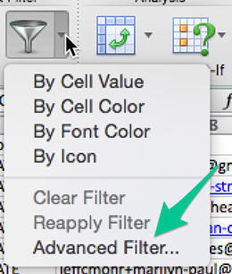
First, select the column you want to find the unique values from. Then click the arrow to the right of the filter button and choose "Advanced Filter..."
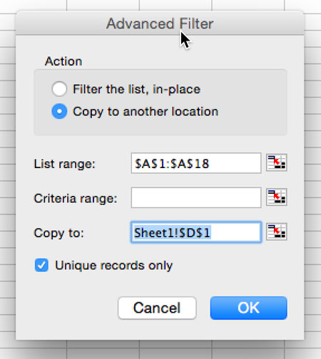
In the next window, choose "Copy to another location", choose where to copy the values to, and then check the box labeled "Unique records only":
You'll now have a listing of all the unique records for that column.
4. The VLOOKUP function
VLOOKUP is great when you have information about a given item spread across multiple sheets. VLOOKUP lets you choose which column to be used as a unique way to match (i.e. a person's full name, an ID of some kind, a project name) and then which column you'd like to pull data from if there is a match. It's also a great way to find whether a given value exists in a larger dataset.
For example, let's say you have a smaller list of people you are mapping and then a huge spreadsheet full of lots of columns of data, only some of which is relevant. You may go through and copy and paste the values or you could save yourself a whole lot of time and frustration by learning to use VLOOKUP.
Consider a spreadsheet with the following structure:
| Label | Type | Description | Phone Number | Organization |
|---|---|---|---|---|
| Bob Jones | Person | |||
| James Gallo | Person | |||
| Jenny Pinsky | Person |
You also have a huge database of contact information that you know probably has records for Bob, James, and Jenny. If you wanted to pull in the phone number for these people automatically, you could use VLOOKUP. The function has the following settings:
=VLOOKUP(lookup_value,table_array,col_index_number, [range_lookup])
- lookup_value: Which value should be used for searching
- table_array: The sheet that you want to search in, make sure the column that has possible matched for the lookup_value is the furthest left column in the selection
- col_index_number: Which column of the table you want to return as the result if a match is found
- range_lookup: Just always include "false" here.
If we had another sheet we were searching in with the following structure:
| Full Name | Employee ID | Location | About | Phone Number |
|---|---|---|---|---|
| Frank Pablo | ||||
| James Gallo | 432-438 | Orland, Florida | James is VP of ... | 408-355-3499 |
| Wilma Deetz |
And we were trying to pull in James' "About" information into the description column, we'd use the following formula:
=VLOOKUP(A3,Sheet2!A:E,4,FALSE)
As with any formula in Excel, just copy it down the column and it will automatically pull in the content. What a time saver!
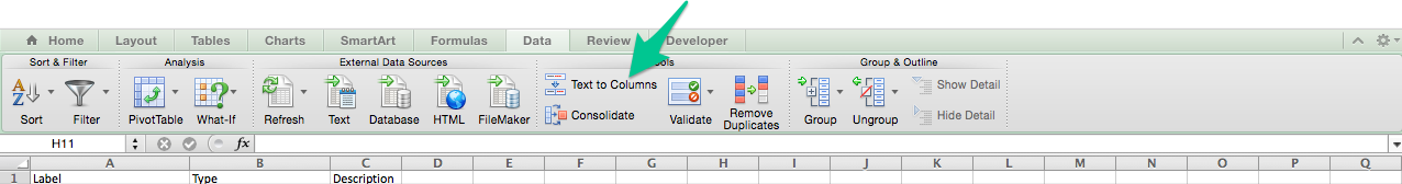
5. Text to columns
Think of text to columns as the sister to the CONCATENATE function. Sometimes you want to put cells together, other times you want to split them apart. The latter is when text to columns becomes useful.
Select the column you'd like to split and then click "Text to Columns" from within the "Data" tab on the Excel ribbon.
You can choose either delimited or fixed width:
- delimited - Useful for when there is a specific character (such as a comma or semicolon) that can be used to split a given cell value.
- fixed - Useful for when you can split a cell a given number of characters in (say if you have a five digit ID on the front of a value that you wanted to split off).
Follow the guidance and then click "Finish" to split the column. Note that you'll need to blank space to the right of the column you are splitting so you don't overwrite other values.
Have another favorite to share?
Use the comments below to contribute a formula, feature, or tool!